Your First Colibri Fit

In this section, we will guide you through the steps to run a fit with a PDF model that is already implemented and readily available within Colibri.

For this exercise, we will be running a Level 0 closure test with the Les Houches parametrisation model, which was implemented in this tutorial.

Make sure you have installed the code first!

Step 1: enable the executable

To run this fit, you will need to be in the right directory:

cd colibri/colibri/examples/les_houches_examples/

You will see that, in this directory, there is a pyproject.py script. This is the script that will allow you to enable the executable for this example, by running the following command in your colibri-dev conda environment:

pip install -e .

You now have access to an executable called les_houches_exe, that you will use to run Les Houches fits.

Step 2: running the closure test

In the colibri/examples/les_houches_example/runcards directory you will find an example runcard called lh_fit_closure_test.yaml. You can find a detailed discussion on this runcard on the tutorial on how to run closure tests. For now, you can simply run this runcard with the following command:

les_houches_exe lh_fit_closure_test.yaml

This step will download the PDF grid LH_PARAM_20250519.

If you don’t have it already, it will also download the theory 40000000.

After you run the fit the first time, any subsequent fits should be faster.

A directory called lh_fit_closure_test, containing the output of the fit, should have been created. You can read more about the fit folders here.

Step 3: Evolving the fit

If you don’t already have it, you will need to download the EKO corresponding to the theory used in this tutorial [CHM22a, CHM22b]:

vp-get EKO 40000000

You can then evolve the fit by running the following command from the les_houches_example directory:

evolve_fit lh_fit_closure_test

You can read more on fit evolution in this section.

Step 4: Generating a validphys report

Finally, you can run:

validphys plot_pdf_fits.yaml

to generate a validphys report [ZCw+25].

The result

As an example, we show the result of the fit for the gluon PDF.

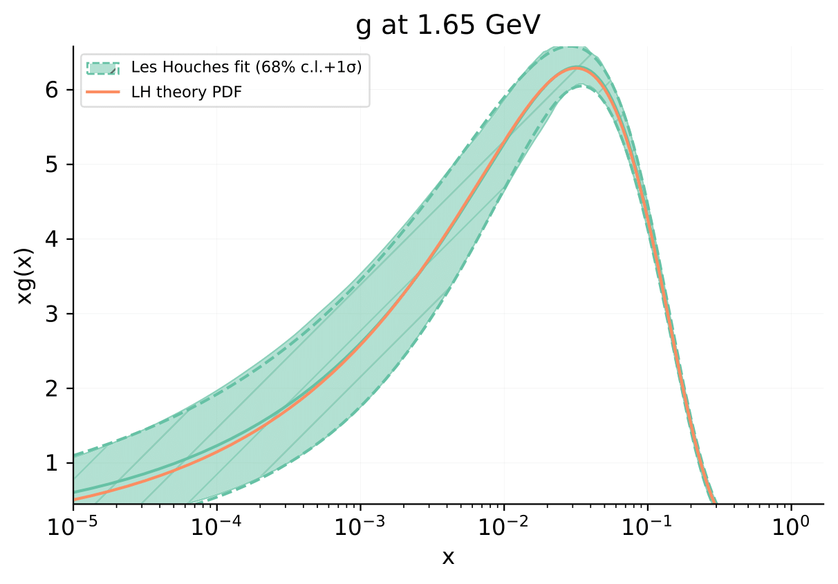
The orange line, labelled LH theory PDF, shows the gluon PDF used to generate the pseudo-data, i.e. the underlying law we are trying to recover. As mentioned above, this was computed using the best-fit values for each parameter, as presented in Ref. A+05. The green curve/section, labelled Les Houches fit 68% c.i. + 1\(\sigma\), shows the result of the closure test fit with error band.