Closure Test
Step 1: enable the executable
The first step is to enable the executable for this tutorial.
In your colibri-dev conda environment, go to the les_houches_example directory,
found in:
cd colibri/examples/les_houches_example
Then run:
pip install -e .
This will enable an executable called les_houches_exe.
Step 2: runcard
In the colibri/examples/les_houches_example/runcards directory you will find
an example runcard called lh_fit_closure_test.yaml, which looks like this:
meta: 'An example fit using Colibri, reduced DIS dataset.'

#######################
# Data and theory specs
#######################

dataset_inputs:
  # DIS
- {dataset: SLAC_NC_NOTFIXED_P_EM-F2, variant: legacy_dw}
- {dataset: SLAC_NC_NOTFIXED_D_EM-F2, variant: legacy_dw}
- {dataset: BCDMS_NC_NOTFIXED_P_EM-F2, variant: legacy_dw}
- {dataset: BCDMS_NC_NOTFIXED_D_EM-F2, variant: legacy_dw}
# - {dataset: CHORUS_CC_NOTFIXED_PB_NU-SIGMARED, variant: legacy_dw}
# - {dataset: CHORUS_CC_NOTFIXED_PB_NB-SIGMARED, variant: legacy_dw}
# - {dataset: NUTEV_CC_NOTFIXED_FE_NU-SIGMARED, cfac: [MAS], variant: legacy_dw}
# - {dataset: NUTEV_CC_NOTFIXED_FE_NB-SIGMARED, cfac: [MAS], variant: legacy_dw}
# - {dataset: HERA_NC_318GEV_EM-SIGMARED, variant: legacy}
# - {dataset: HERA_NC_225GEV_EP-SIGMARED, variant: legacy}
# - {dataset: HERA_NC_251GEV_EP-SIGMARED, variant: legacy}
# - {dataset: HERA_NC_300GEV_EP-SIGMARED, variant: legacy}
# - {dataset: HERA_NC_318GEV_EP-SIGMARED, variant: legacy}
# - {dataset: HERA_CC_318GEV_EM-SIGMARED, variant: legacy}
# - {dataset: HERA_CC_318GEV_EP-SIGMARED, variant: legacy}
# - {dataset: HERA_NC_318GEV_EAVG_CHARM-SIGMARED, variant: legacy}
# - {dataset: HERA_NC_318GEV_EAVG_BOTTOM-SIGMARED, variant: legacy}
# - {dataset: NMC_NC_NOTFIXED_EM-F2, variant: legacy_dw}
# - {dataset: NMC_NC_NOTFIXED_P_EM-SIGMARED, variant: legacy}


theoryid: 40000000                     # The theory from which the predictions are drawn.
use_cuts: internal                     # The kinematic cuts to be applied to the data.

closure_test_level: 0                  # The closure test level: False for experimental, level 0
                                       # for pseudodata with no noise, level 1 for pseudodata with
                                       # noise.

closure_test_pdf: LH_PARAM_20250519  # The closure test PDF used if closure_test_level is not False

#####################
# Loss function specs
#####################

positivity:                            # Positivity datasets, used in the positivity penalty.
  posdatasets:
  - {dataset: NNPDF_POS_2P24GEV_F2U, variant: None, maxlambda: 1e6}

positivity_penalty_settings:
  positivity_penalty: false
  alpha: 1e-7
  lambda_positivity: 0

# Integrability Settings
integrability_settings:
  integrability: False

use_fit_t0: True                       # Whether the t0 covariance is used in the chi2 loss.
t0pdfset: NNPDF40_nnlo_as_01180         # The t0 PDF used to build the t0 covariance matrix.


###################
# Methodology specs
###################
prior_settings:
  prior_distribution: uniform_parameter_prior
  prior_distribution_specs:
    bounds:
      alpha_gluon: [-0.1, 1]
      beta_gluon: [9, 13]
      alpha_up: [0.4, 0.9]
      beta_up: [3, 4.5]
      epsilon_up: [-3, 3]
      gamma_up: [1, 6]
      alpha_down: [1, 2]
      beta_down: [8, 12]
      epsilon_down: [-4.5, -3]
      gamma_down: [3.8, 5.8]
      norm_sigma: [0.1, 0.5]
      alpha_sigma: [-0.2, 0.1]
      beta_sigma: [1.2, 3]


# Nested Sampling settings
ns_settings:
  sampler_plot: true
  n_posterior_samples: 100      # Number of posterior samples generated.
  ReactiveNS_settings:
    vectorized: False
    ndraw_max: 500              # Maximum number of points to simultaneously propose.
  Run_settings:
    min_num_live_points: 200    # Minimum number of live points throughout the run.
    min_ess: 50                 # Target number of effective posterior samples.
    frac_remain: 0.3            # Integrate until this fraction of the integral is left in the remainder.
  SliceSampler_settings:
    nsteps: 106                 # number of accepted steps until the sample is considered independent.


actions_:
- run_ultranest_fit                      # Choose from ultranest_fit, monte_carlo_fit, analytic_fit
TODO: add some discussion on the runcard
Step 3: producing the fit
To produce the fit, run the following command from the colibri/les_houches_example
directory:
les_houches_exe runcards/lh_fit_closure_test.yaml
This step will download the PDF grid LH_PARAM_20250429, which has been produced
by computing the relevant PDFs for the Les Houches model (see Les Houches Parametrisation) with
the best-fit values for the parameters, taken from Ref. [A+05].
If you don’t have it already, it will also download the theory
40000000.
After you run the fit the first time, any subsequent times should take less than 3 minutes.
A directory called lh_fit_closure_test, containing the output of the fit,
should have been created.
3.1 Evolving the fit
If you don’t already have it, you will need to download the EKO corresponding to the theory used in this tutorial;
vp-get eko 40000000
TODO: add link to EKO NNPDF documentation
You can evolve the fit by running the following command from the les_houches_example
directory:
evolve_fit lh_fit_closure_test
3.2 Generating a validphys report
Finally, you can run:
validphys plot_pdf_fits.yaml
to generate a validphys report.
The result
As an example, we show the result of the fit for the gluon PDF.
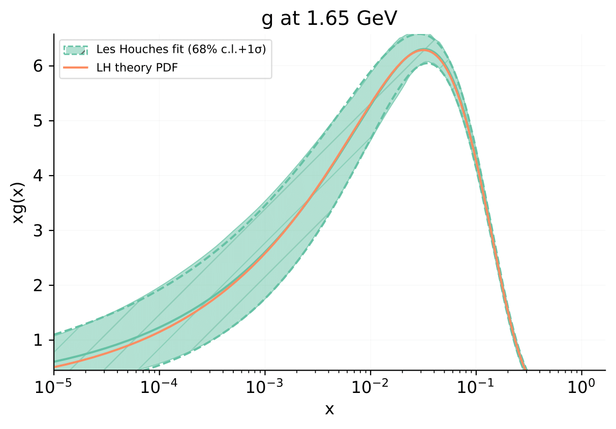
The orange line, labelled LH theory PDF, shows the gluon PDF computed from best-fit values for all parameters. The green curve/section, labelled Les Houches fit 68% c.i. + 1\(\sigma\), shows the result of the fit with error band.