Features#
Here we detail some of the main features and capabilities of the \(\text{SIMUnet}\) methodology.
PDF and SMEFT fits#
\(\text{SIMUnet}\) can perform simultaneous PDF-SMEFT fits. The interplay between PDFs and SMEFT parameters is complex and traditional methods of treating them separately can lead to inconsistencies and inaccuracies. By performing simultaneous fits, the \(\text{SIMUnet}\) framework addresses this challenge head-on, ensuring that the subtleties and interdependencies are correctly captured.
In Fig. 1 we show an example of a PDF obtained from a simultaneous PDF-SMEFT fit with \(\text{SIMUnet}\) and compare it its analogous SM result.

Figure 1: Gluon PDF determined from a simultaneous PDF-SMEFT fit (green) and a SM (NNPDF4.0) fit (blue) in the top sector. We also show the PDF obtained when no top data is included in the SM fit.#
We see how the inclusion of new data shifts the SM PDF, and the impact of performing a simultaneous PDF-SMEFT fit which, in this case, allows the PDF to accommodate better the inclusion of new data.
Additionally, \(\text{SIMUnet}\) provides distributions of SMEFT coefficients, as shown in Fig. 2.
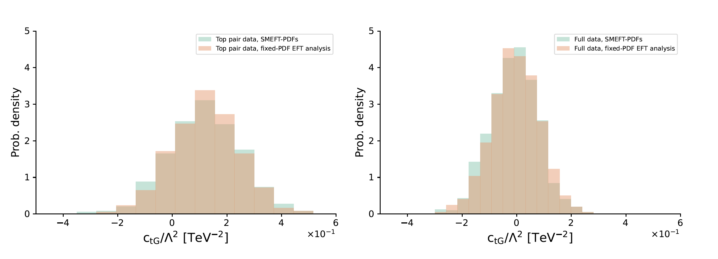
Figure 2: Distribution of the \(c_{tG}\) SMEFT coefficient determined from a simultaneous PDF-SMEFT fit (green) and a fixed-PDF fit (orange).#
In this case, the distribution of the SMEFT coefficient \(c_{tG}\) changes mildly. The PDF-SMEFT interplay is not trivial, and in other cases more substantial changes can be found.
\(\text{SIMUnet}\) also provides complete summaries to show the behaviour of the SMEFT basis as a whole. In Fig. 3, we show a plot with the bounds for a set of top operators.
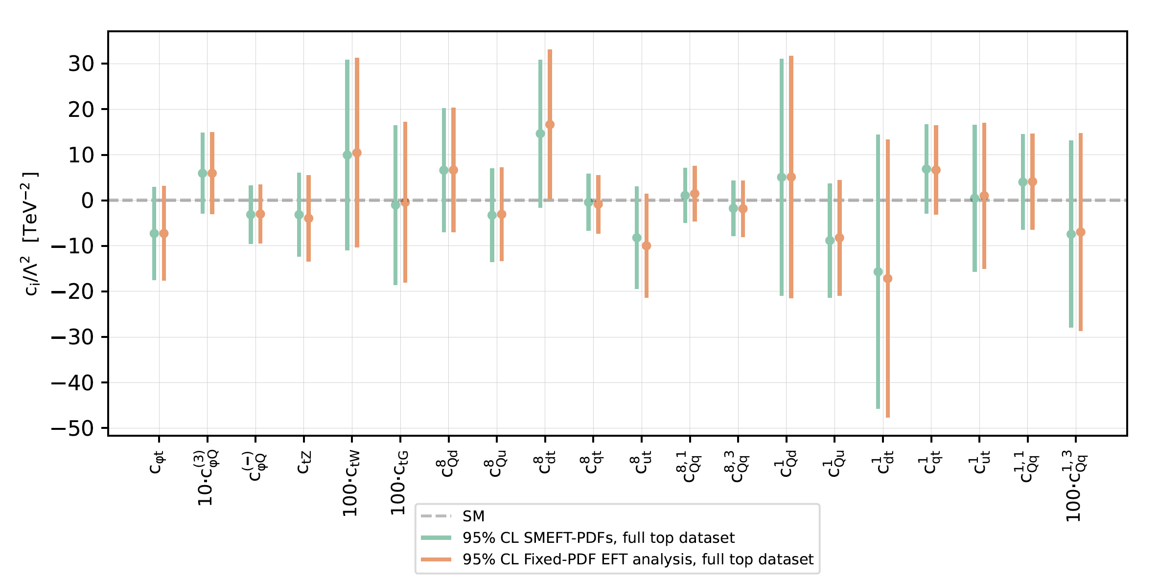
Figure 3: Bounds for a set of 20 SMEFT operators obtained with \(\text{SIMUnet}\) in a simultaneous PDF-SMEFT fit and a fixed-PDF fit.#
\(\text{SIMUnet}\) also provides summary tables, correlations, PCA, among many other things.
The \(\text{SIMUnet}\) methodology can also obtain the correlation between SMEFT coefficients and PDFs, as shown in Fig. 4. Correlations like the one shown below can be useful to quantify the strength of the PDF-SMEFT interplay when performing simultaneous and fixed-PDF fits.
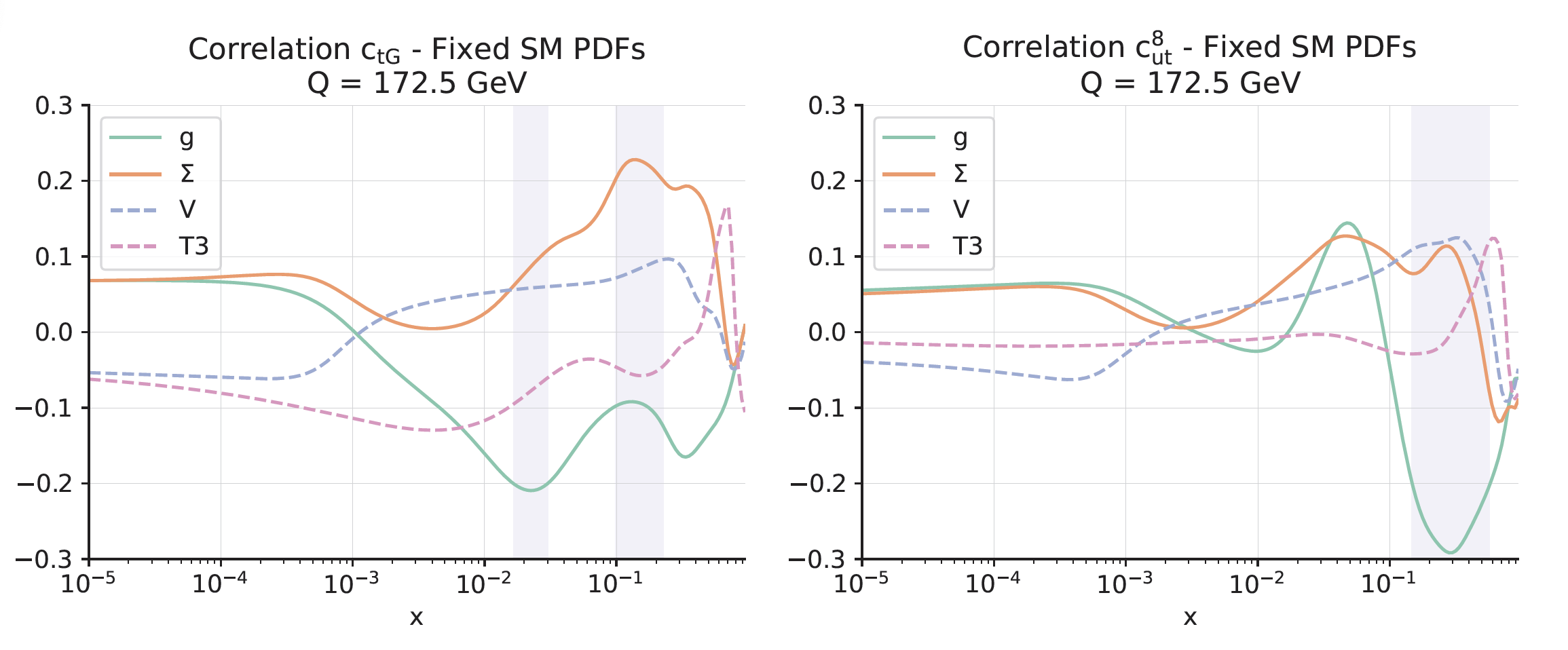
Figure 4: Correlations between the SMEFT coefficients \(c_{tG}\) and \(c_{ut}^{8}\) and the PDFs of the gluon and some components of the evolution basis.#
Can PDFs absorb new physics?#
\(\text{SIMUnet}\) also allows the user to determine if PDFs can absorb new physics by ‘injecting’ new physics into the generation of pseudodata that is then used to fit the PDFs.
As an example, we can consider the well known oblique parameters \(W\) and \(Y\), which can parametrise new physics affecting Drell-Yan processes and DIS. With \(\text{SIMUnet}\), we contaminate the data by using several values, as shown in Fig. 5.
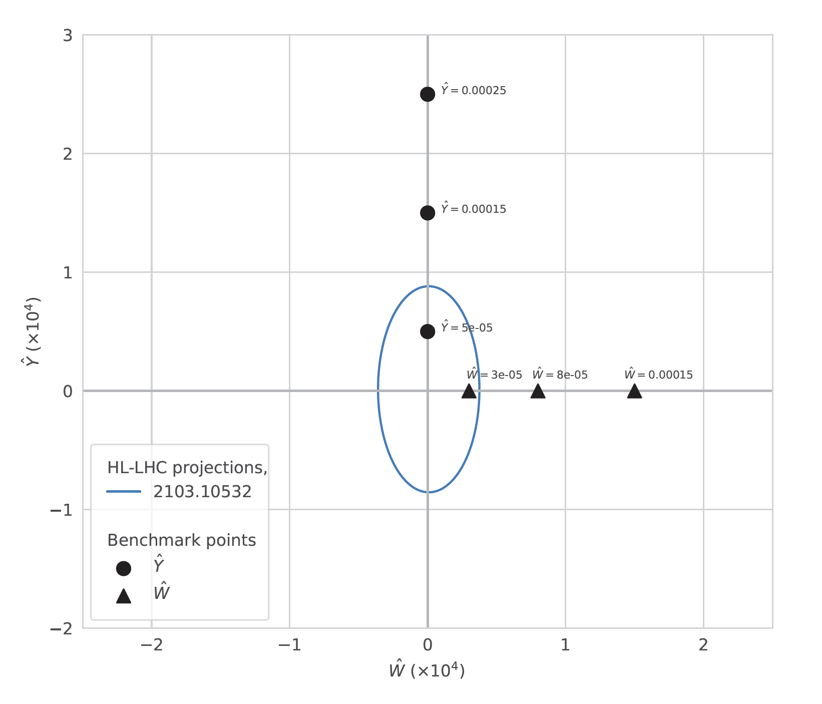
Figure 5: Values of \(W\) and \(Y\) used to inject new physics in the data that goes into the fit to assess the possible contamination of the PDFs by new physics.#
\(\text{SIMUnet}\) higlights an important issue that affects the search for new physics in this case. In the plot above, the points \(W = 8 \times 10^{-5}\) is beyond current bounds. The injection of this new physics does not deteriorate the fit quality in a global fit, and therefore it is not spotted. However, as shown in Fig. 6, the PDF luminosities shift significantly.
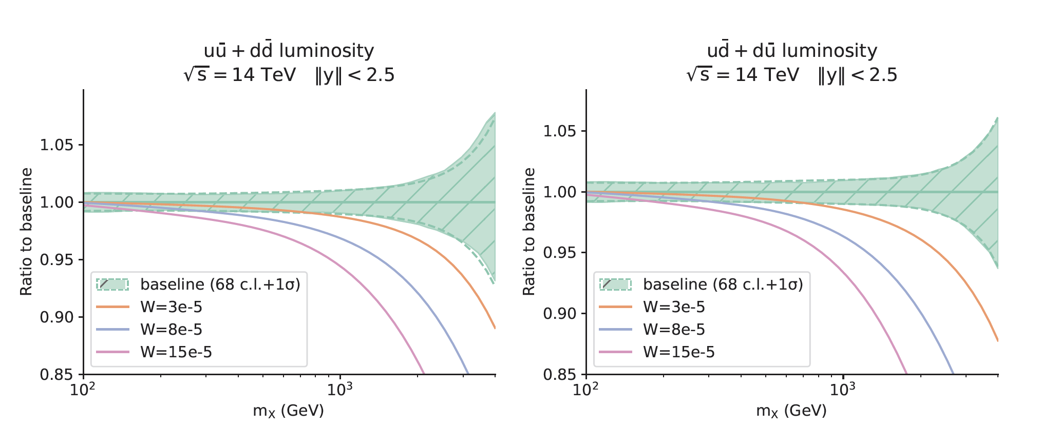
Figure 6: Shift in the PDF luminosities with different values of new physics.#
In this way, \(\text{SIMUnet}\) determines that there is enough flexibility in the fit to absorb the \(W = 8 \times 10^{-5}\) value in the PDFs. Using these ‘contaminated’ PDFs can lead to biased predictions and, in extreme cases, detects new physics where there is none. In Fig. 7, we show the predictions for \(W^{+} H\) production, which is not affected by the injection of new physics, obtained using the contaminated PDF set.
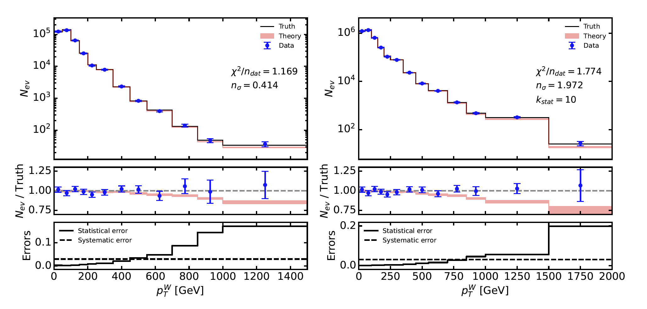
Figure 7: Projections for \(W^+ H\) production using the contaminated PDFs. Left: HL-LHC, Right: HL-LHC with enhanced statistics.#
We have discussed some of the capabilities of the \(\text{SIMUnet}\) metholodgy. Further information can be found in the other sections of this documentation and in the original references.
